1000 Genomes Project Metadata • kgp

This kgp data package provides metadata about populations and data about samples from the 1000 Genomes Project, including the 2,504 samples sequenced for the Phase 3 release and the expanded collection of 3,202 samples with 602 additional trios.

Installation

You can install the released version of kgp from CRAN with:

install.packages("kgp")

You can install the development version of kgp from GitHub with:

# install.packages("devtools")
devtools::install_github("stephenturner/kgp")

About the data

The 1000 Genomes Project data Phase 3 data contains 2,504 samples with sequence data available, and was later expanded to 3,202 samples with high coverage adding 602 trios. Data is available through the 1000 Genomes FTP site and GitHub.

Pilot publication: An integrated map of genetic variation from 1,092 human genomes
Phase 1 publication: A map of human genome variation from population scale sequencing
Phase 3 publication: A global reference for human genetic variation
Expanded high-coverage publication: High-coverage whole-genome sequencing of the expanded 1000 Genomes Project cohort including 602 trios

There are three data sets available in the kgp package.

library(kgp)
data(kgp)

The kgp3 data contains pedigree and population information for the 2,504 samples included in the Phase 3 release of the 1000 Genomes Project data.

kgp3
#> # A tibble: 2,504 × 10
#>    fid     id      pid   mid     sex sexf   pop   reg   population        region
#>    <chr>   <chr>   <chr> <chr> <int> <fct>  <chr> <chr> <chr>             <chr> 
#>  1 HG00096 HG00096 0     0         1 male   GBR   EUR   British in Engla… Europe
#>  2 HG00097 HG00097 0     0         2 female GBR   EUR   British in Engla… Europe
#>  3 HG00099 HG00099 0     0         2 female GBR   EUR   British in Engla… Europe
#>  4 HG00100 HG00100 0     0         2 female GBR   EUR   British in Engla… Europe
#>  5 HG00101 HG00101 0     0         1 male   GBR   EUR   British in Engla… Europe
#>  6 HG00102 HG00102 0     0         2 female GBR   EUR   British in Engla… Europe
#>  7 HG00103 HG00103 0     0         1 male   GBR   EUR   British in Engla… Europe
#>  8 HG00105 HG00105 0     0         1 male   GBR   EUR   British in Engla… Europe
#>  9 HG00106 HG00106 0     0         2 female GBR   EUR   British in Engla… Europe
#> 10 HG00107 HG00107 0     0         1 male   GBR   EUR   British in Engla… Europe
#> # … with 2,494 more rows
#> # ℹ Use `print(n = ...)` to see more rows

The kgpe data contains pedigree and population information all 3,202 samples included in the expanded 1000 Genomes Project data, which includes 602 trios.

kgpe
#> # A tibble: 3,202 × 11
#>    fid     id      pid   mid     sex sexf   pop   reg   population region phase3
#>    <chr>   <chr>   <chr> <chr> <int> <fct>  <chr> <chr> <chr>      <chr>  <lgl> 
#>  1 HG00096 HG00096 0     0         1 male   GBR   EUR   British i… Europe TRUE  
#>  2 HG00097 HG00097 0     0         2 female GBR   EUR   British i… Europe TRUE  
#>  3 HG00099 HG00099 0     0         2 female GBR   EUR   British i… Europe TRUE  
#>  4 HG00100 HG00100 0     0         2 female GBR   EUR   British i… Europe TRUE  
#>  5 HG00101 HG00101 0     0         1 male   GBR   EUR   British i… Europe TRUE  
#>  6 HG00102 HG00102 0     0         2 female GBR   EUR   British i… Europe TRUE  
#>  7 HG00103 HG00103 0     0         1 male   GBR   EUR   British i… Europe TRUE  
#>  8 HG00105 HG00105 0     0         1 male   GBR   EUR   British i… Europe TRUE  
#>  9 HG00106 HG00106 0     0         2 female GBR   EUR   British i… Europe TRUE  
#> 10 HG00107 HG00107 0     0         1 male   GBR   EUR   British i… Europe TRUE  
#> # … with 3,192 more rows
#> # ℹ Use `print(n = ...)` to see more rows

The kgpmeta contains population metadata for the 26 populations across five continental regions.

kgpmeta
#> # A tibble: 26 × 7
#>    pop   population                          reg   region   regco…¹   lat    lng
#>    <chr> <chr>                               <chr> <chr>    <chr>   <dbl>  <dbl>
#>  1 CDX   Chinese Dai in Xishuangbanna, China EAS   East As… #778500  22   101.  
#>  2 CHB   Han Chinese in Bejing, China        EAS   East As… #778500  39.9 116.  
#>  3 JPT   Japanese in Tokyo, Japan            EAS   East As… #778500  35.7 140.  
#>  4 KHV   Kinh in Ho Chi Minh City, Vietnam   EAS   East As… #778500  10.8 107.  
#>  5 CHS   Southern Han Chinese, China         EAS   East As… #778500  23.1 113.  
#>  6 BEB   Bengali in Bangladesh               SAS   South A… #c44cfd  23.7  90.4 
#>  7 GIH   Gujarati Indian in Houston,TX       SAS   South A… #c44cfd  29.8 -95.4 
#>  8 ITU   Indian Telugu in the UK             SAS   South A… #c44cfd  52.5  -1.89
#>  9 PJL   Punjabi in Lahore,Pakistan          SAS   South A… #c44cfd  31.6  74.4 
#> 10 STU   Sri Lankan Tamil in the UK          SAS   South A… #c44cfd  52.5  -1.89
#> # … with 16 more rows, and abbreviated variable name ¹regcolor
#> # ℹ Use `print(n = ...)` to see more rows

Examples

library(dplyr)
library(ggplot2)
library(kgp)
data(kgp)

Count the number of samples in each region, or in each population:

kgp3 %>% 
  count(region) %>% 
  knitr::kable()

region	n
Africa	661
America	347
East Asia	504
Europe	503
South Asia	489

kgp3 %>% 
  count(region, population) %>% 
  knitr::kable()

region	population	n
Africa	African Ancestry in Southwest US	61
Africa	African Caribbean in Barbados	96
Africa	Esan in Nigeria	99
Africa	Gambian in Western Division, The Gambia	113
Africa	Luhya in Webuye, Kenya	99
Africa	Mende in Sierra Leone	85
Africa	Yoruba in Ibadan, Nigeria	108
America	Colombian in Medellin, Colombia	94
America	Mexican Ancestry in Los Angeles, California	64
America	Peruvian in Lima, Peru	85
America	Puerto Rican in Puerto Rico	104
East Asia	Chinese Dai in Xishuangbanna, China	93
East Asia	Han Chinese in Bejing, China	103
East Asia	Japanese in Tokyo, Japan	104
East Asia	Kinh in Ho Chi Minh City, Vietnam	99
East Asia	Southern Han Chinese, China	105
Europe	British in England and Scotland	91
Europe	Finnish in Finland	99
Europe	Iberian populations in Spain	107
Europe	Toscani in Italy	107
Europe	Utah residents with Northern and Western European ancestry	99
South Asia	Bengali in Bangladesh	86
South Asia	Gujarati Indian in Houston,TX	103
South Asia	Indian Telugu in the UK	102
South Asia	Punjabi in Lahore,Pakistan	96
South Asia	Sri Lankan Tamil in the UK	102

kgp3 %>% 
  count(region, population) %>% 
  arrange(region, n) %>% 
  mutate(population=forcats::fct_inorder(population)) %>% 
  ggplot(aes(population, n)) + 
  geom_col(aes(fill=region)) + 
  labs(fill=NULL, x=NULL, x="N") + 
  coord_flip() + 
  theme_bw() + 
  theme(legend.position="bottom")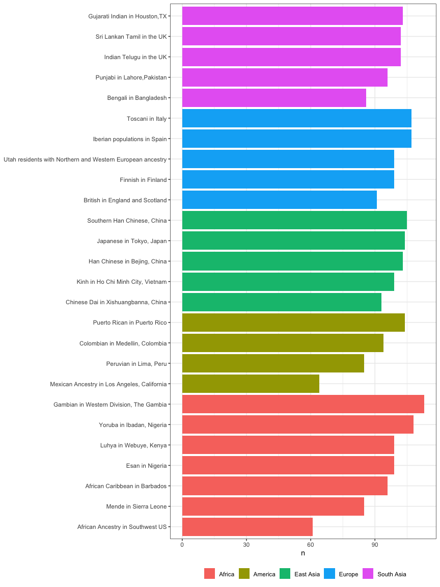

The latitude and longitude coordinates in kgpmeta can be used to plot a map of the locations of the 1000 Genomes populations. There is also a column for region color, which provides a hexadecimal color code to enable reproduction of the population data map as shown on the IGSR population data page. The figure below shows a static map produced using ggplot2, but interactive maps such as that shown on the IGSR population data portal can be created with the leaflet package.

pal <- kgpmeta %>% distinct(reg, regcolor) %>% tibble::deframe()
ggplot() + 
  geom_polygon(data=map_data("world"), 
               aes(long, lat, group=group), 
               col="gray30", fill="gray95", lwd=.2, alpha=.5) + 
  geom_point(data=kgpmeta, aes(lng, lat, col=reg), size=4) + 
  scale_colour_manual(values=pal) +
  theme_minimal() + 
  theme(axis.ticks = element_blank(), 
        axis.text = element_blank(), 
        axis.title = element_blank(), 
        legend.title = element_blank(),
        panel.grid = element_blank(),
        legend.position = "bottom")

Map showing locations of the 1000 Genomes Phase 3 populations.

The table below shows a selection of samples from kgpe showing pedigree information for each sample. This pedigree information could be used in downstream analysis to filter out related individuals, select only trios, or to visualize family structure.

kgpe %>% 
  filter(pid!="0" & mid!="0") %>% 
  group_by(pop) %>% 
  slice(1) %>% 
  head(12) %>% 
  arrange(reg, pop) %>% 
  select(fid:reg) %>% 
  select(-sexf) %>% 
  knitr::kable()

fid	id	pid	mid	sex	pop	reg
BB01	HG01881	HG01879	HG01880	2	ACB	AFR
2367	NA19702	NA19700	NA19701	1	ASW	AFR
NG06	HG02924	HG02923	HG02922	1	ESN	AFR
GB15	HG02463	HG02461	HG02462	1	GWD	AFR
SL02	HG03056	HG03054	HG03055	1	MSL	AFR
CLM03	HG01114	HG01112	HG01113	2	CLM	AMR
SH001	HG00405	HG00403	HG00404	2	CHS	EAS
VN046	HG02015	HG02017	HG02016	1	KHV	EAS
1341	NA06991	NA06993	NA06985	2	CEU	EUR
IBS001	HG01502	HG01500	HG01501	1	IBS	EUR
BD01	HG03008	HG03006	HG03007	1	BEB	SAS
IT002	HG03719	HG03725	HG03722	2	ITU	SAS

The figure below shows an example of a pedigree plot made by parsing the pedigree information using skater and plotting using kinship2. The skater package provides documentation, examples, and a vignette demonstrating how to iteratively plot all pedigrees in a given data set.

kgpe %>% 
  filter(fid=="13291") %>% 
  transmute(fid, id, dadid=pid, momid=mid, sex, affected=1) %>% 
  skater::fam2ped() %>% 
  pull(ped) %>% 
  purrr::pluck(1) %>% 
  kinship2::plot.pedigree(mar=c(4,2,4,2), cex=.8)

Trios in 1000 Genomes Project family 13291.